Project Link: pp.bryanchan.org
(Some) source code: github.com/brrryry/pp
(I really need to add more visuals for my math stuff...)

Yeah...this title is gas.

I recently hit a 5-digit rank in osu, and I still haven't been able to deploy a full coding project despite my idea bank being filled to the brim. The idea that I got the farthest with was the Osu! Beatmap Generator, but I found out that this has already been done. Since I was out of ideas, I decided to just...play more osu.

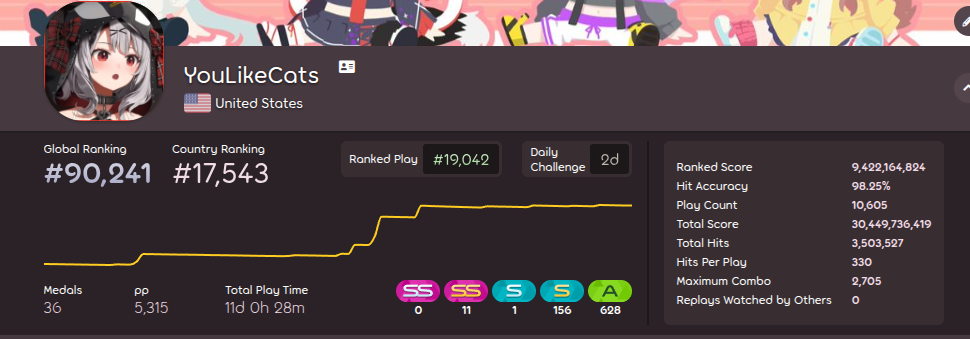
New milestone achieved! :D

While doing this, I used a few different websites to help me get better at the game. One that stood out to me was the osu! skillset analyzer _[1] made by user Kumokoni _[2]. This website scans your top 200 plays, pinned scores, recent plays, and your favorite maps. Then, it calculates a 12-axis user skill portfolio.

My skillset analyzer result. (source)

This website is fantastic, and I have no complaints. It has a very slick UI, and the portfolio is explained EXTREMELY well. It inspired me to look a little bit deeper. What if we could try to recommend maps, but based on axis-free embeddings?

When I talk about "axis-free", I'm referring to the removal of the 12-axis classification. After scrolling through quite a few forums, I found that different people have different ideas of what defines an "axis" of skill. Some examples may include:

So, what if we didn't use any axes to remove disparity? That's what this project aims to do. Without further ado...

---

PP Recommender

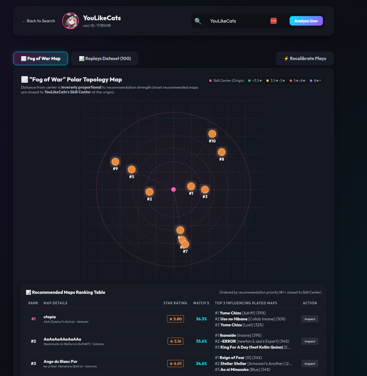
A brief showcase (source)

This website takes username inputs and fetches some top/recent osu replays. Using these replays, it will recommend maps for the user to play.

By definition, it's hard to show the user why a certain map is recommended. Since we don't have explicit skill tags, we can't really say "map X has high aim difficulty" or "map Y has high stream difficulty." Instead, we rely on the map's properties like star rating, accuracy, length, etc. as a proxy for difficulty. This model "learns" the difficulty of the map.

What we CAN do is show the user which maps have similar embeddings to the maps they've played.

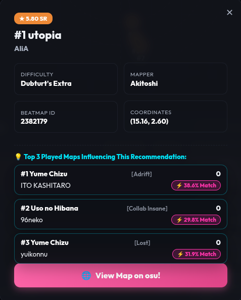
Example of a map recommendation.

While there is the obvious con of not being able to explain why a map is recommended, there are a few pros to this approach:

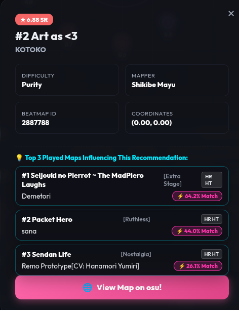
Example of a modded map recommendation for mrekk. Since the influential maps are modded, the model recommends other maps (in modded settings).

In a way, this kind of model has higher potential for better recommendations since we don't rely on multiple subjective axis definitions.

Additionally, the website allows you to view the replays that are being used to calculate your recommendations.

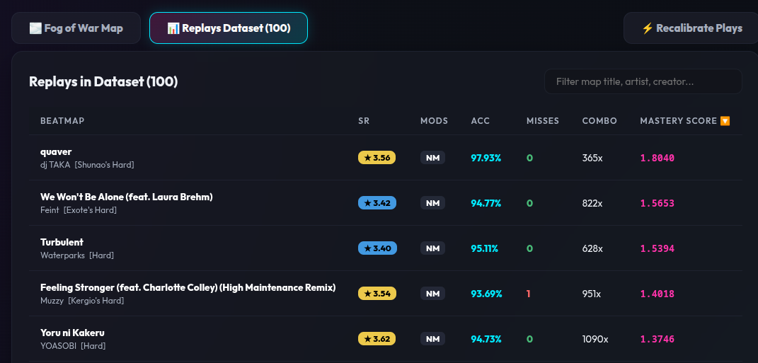
Example of the replay list

This is a really simple website, but there's a lot of room for expansion. Some ideas I had include:

There's also a lot of bugs at the moment that need to be fixed. To be honest, I vibe-coded a lot of the frontend, and the backend can still be improved in terms of efficiency. That being said, I wanted to deploy an MVP as fast as possible to get it into the hands of other players and get their feedback.

That's really it for the showcase. If you don't want to read my yap on the technical details, the blog basically ends here. Thank you for checking in :)

---

The Models

Oh boy. There's a bunch of math-heavy stuff to unpack here, and it may be hard to read in one sitting (because I can't write concisely).

I'd recommend having a background in linear algebra, calculus, and probability to fully understand this section.

Here's a brief idea of the topic list:

To start, let's talk about how I inputted my data.

1. Data Processing

Osu! beatmap files (.osu files) have a specific format. From them, you can extract all the hit objects (circles, sliders and spinners). You can also get all the timing points (determines bpm, offset, slider velocity, etc.).

To put this data into a nice list of numbers, I did the following:

All in all, I had a 13-dimensional vector.

I took a maximum of 2000 objects per map to keep the padding and training time reasonable. Thus, our input is a matrix of size 2000x13.

---

2. Variational Autoencoder (VAE) Math _[3]

If you want to skip all the math, click here.

The variational autoencoder is a model that was introduced around 2013 by Diedrik P. Kingma and Max Welling. The paper can be found here _[4].

Standard autoencoders have two parts: an encoder, and a decoder. The encoder turns an input vector (list of numbers) into a compressed vector (basically shrinking the input vector in size, i.e. dimensions). The decoder tries to reconstruct the original input from this compressed vector. An easy way to think about it is trying to compress a file into a zip file, and then decompressing the zip file. (Note: This is not actually how zip files work, but it's a good analogy.)

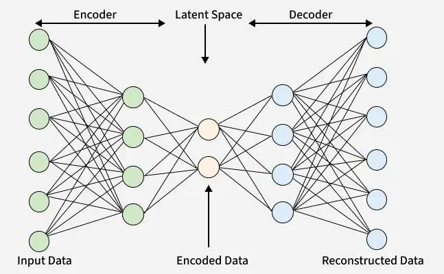
A diagram of an autoencoder (NOT A VAE) from GeeksforGeeks [5]. (source)

In most cases, both the encoder and decoder are defined as multilayer perceptrons (fancy term for a type of neural network). Let's use a more mathematical approach (this will make it easier to compare VAEs later).

1. Mathematical Formulation of Autoencoders

Given an input vector $x \in \mathbb{R}^d$, we create the encoder function $f_\phi$ which maps $x$ to a compressed vector $z \in \mathbb{R}^d$ ($d << D$).

(The notation $f_\phi$ means that we have a function $f$ that depends on parameters $\phi$. In this case, $\phi$ represents the weights and biases of the neural network.)

We use the decoder function $g_\theta$ to reconstruct an estimation of the original vector $\hat{x}$.

Our goal is to learn parameters $\phi$ and $\theta$ such that $\hat{x} \approx x$. In the event of continuous output space (like our map features), we can define our reconstruction loss $L_{rec}(\phi, \theta)$ using Mean Squared Error _[20] (a typical deterministic loss function for regression tasks):

Autoencoders can be trained like any other neural network, so gradient descent is typically used.

That's how standard autoencoders work, but variational autoencoders are a bit different. Variational Autoencoders approach learning with a more probabilistic approach (specifically using Bayesian Inference _[6]).

2. Maximum Likelihood Estimation _[7] - A Primer

📊 Click here for more info!

Small tangent (I promise it's relevant), but do you know how statistics like sample mean and sample standard deviation are derived? I'm sure you've heard of them before.

If you have a i.i.d _[12] normally distributed _[18] random sample of data, say points $x_1, x_2, \dots, x_n$, we can calculate the sample mean $\bar{x}$ as:

$$\bar{x} = \frac{1}{n} \sum_{i=1}^{n} x_i$$

This formula is beautifully simple, and it's built on the idea that we can maximize the chance of getting our sample data given a certain distribution.

As an analogy, think of flipping a coin. If the coin is truly fair (50/50), what's the probability of getting 3 heads in a row? The same idea goes here - if the true population mean is $\mu$, what's the probability of getting our sample data? We want to choose a $\mu$ that maximizes this probability.

To figure this out, we use the Maximum Likelihood Estimation (MLE) method - a method for estimating the parameters of a statistical model given an observed dataset.

I'll spare the calculus lesson (do you know derivatives/integrals?), but let's go through an example.

We will make an estimation of the population mean $\mu$. We will call our estimate $\hat{\mu}$ (mu-hat).

We look at the likelihood of observing our data given the parameter $\mu$ (the chance that we get this data if the mean is $\mu$). If each data point is sampled independently, then the likelihood of observing all of our data is the product of the likelihoods of observing each data point.

$$L(\mu) = P(X | \mu) = \prod_{i=1}^{n} \frac{1}{\sqrt{2\pi\sigma^2}} e^{-\frac{(x_i - \mu)^2}{2\sigma^2}}$$

The formula above looks ridiculous, and it looks like I pulled it out of thin air, but it's the normal probabilty density function. Now that I'm writing this, I realize that there's a lot to explain...oof...

Typically, we use log-likelihood (taking the logarithm) to make computations easier.

$$\begin{align} l(\mu) &= log(\prod_{i=1}^{n} \frac{1}{\sqrt{2\pi\sigma^2}} e^{-\frac{(x_i - \mu)^2}{2\sigma^2}}) \\ &= \sum_{i=1}^{n} log(\frac{1}{\sqrt{2\pi\sigma^2}}) + log(e^{-\frac{(x_i - \mu)^2}{2\sigma^2}}) \\ &= \sum_{i=1}^{n} -log(\sqrt{2\pi\sigma^2}) - \frac{(x_i - \mu)^2}{2\sigma^2} \end{align}$$

Now, how do we maximize $l(\mu)$? We find the critical point (calculus 1)! Since we know that the function is concave (you can verify this by taking the Hessian of the function, but just take my word for it...), the critical point is guaranteed to be the maximum.

By differentiating the log-likelihood function with respect to $\mu$, we get:

$$\begin{align} \frac{d}{d\mu} [l(\mu)] &= \frac{d}{d\mu} \left[ \sum_{i=1}^{n} -log(\sqrt{2\pi\sigma^2}) - \frac{(x_i - \mu)^2}{2\sigma^2} \right] \\ &= \sum_{i=1}^{n} \frac{d}{d\mu} [-log(\sqrt{2\pi\sigma^2})] - \frac{d}{d\mu} \left[ \frac{(x_i - \mu)^2}{2\sigma^2} \right] \\ &= 0 - \frac{1}{2\sigma^2} \sum_{i=1}^{n} 2(x_i - \mu)(-1) \\ &= \frac{1}{\sigma^2} \sum_{i=1}^{n} (x_i - \mu) \end{align}$$

And by setting it to 0, we solve for our estimator $\hat{\mu}$:

$$\begin{gathered} \frac{1}{\sigma^2} \sum_{i=1}^{n} (x_i - \hat{\mu}) = 0 \\ \sum_{i=1}^{n} (x_i - \hat{\mu}) = 0 \\ \sum_{i=1}^{n} x_i - \sum_{i=1}^{n} \hat{\mu} = 0 \\ \sum_{i=1}^{n} x_i = n \hat{\mu} \\ \hat{\mu} = \frac{1}{n} \sum_{i=1}^{n} x_i = \bar{x} \end{gathered}$$

Therefore, our best estimation for the population mean is $\bar{x}$, commonly known as the sample mean!

I wish I learned how these formulas were derived back when I first took statistics...it's honestly fascinating.

3. Bayesian Inference _[6] - Another Primer

🔮 Click here for more info!

To understand VAEs, we must first understand how Bayesian Inference _[6] works in the context of statistics.

This technique involves using a prior belief (a hypothesis $H$), and using new evidence (data $D$) to update our beliefs (the posterior probability $P(H|D)$).

We begin with Bayes' Theorem _[8] - a way to calculate posterior probabilities. Bayes' Theorem is defined as:

$$P(H|D) = \frac{P(D|H)P(H)}{P(D)}$$

Where:

• $H$: Hypothesis - A statement or proposition about the world
• $D$: Data - The observed evidence
• $P(H|D)$: Posterior Probability - The probability of the hypothesis being true given the data
• $P(D|H)$: Likelihood - The probability of the observed data given the hypothesis
• $P(H)$: Prior Probability - The probability of the hypothesis being true before observing the data
• $P(D)$: Evidence - The probability of the observed data

In MLE, we treated the hypothesis (or parameters) as fixed, unknown constants, and our goal was to find the single value that maximized the likelihood $P(D|H)$ of our observed data (for example, finding the MLE of $\mu$ - a CONSTANT).

In the Bayesian framework, however, we treat the hypothesis (i.e. $\mu$) itself as a random variable. We assign it a prior probability distribution $P(\mu)$ (representing our beliefs before seeing any data). For instance, maybe we think that coin flips are usually fair, so we assign a prior probability distribution that is peaked around $\mu = 0.5$ (we do not say that $\mu$ IS 0.5 - this is the difference).

We then update our beliefs by multiplying the prior by the likelihood $P(D|\mu)$ to get the posterior probability distribution $P(\mu|D)$ using Bayes' Theorem.

Here's an interesting way to think about it: MLE is basically Bayes' rule with a uniform prior distribution ($P(H)$ = 1 for all H).

4. Inferring Posterior Distributions (Primers Over!)

We apply the Bayesian framework to infer the posterior probability distribution $P(z|x)$:

Where:

• $P(z|x)$: Posterior Probability - The probability of the latent variable given the observed data
• $P(x|z)$: Likelihood - The probability of the observed data given the latent variable
• $P(z)$: Prior Probability - The probability of the latent variable before observing the data
• $P(x)$: Evidence - The probability of the observed data

At the same time, we want to infer the posterior distribution $P(z|x)$ to find the latent representation $z$ for any given data point $x$.

(TLDR: we want to maximize the likelihood of our vector $x$ while finding a compressed form $z$ that captures the most important features in $x$.)

To apply this to our autoencoder, we parameterize the generative model (the decoder) with parameters $\theta$. Thus, our model's likelihood is $P_\theta(x|z)$ and the joint distribution is $P_\theta(x, z) = P_\theta(x|z)P(z)$ (assuming a fixed prior $P(z)$).

As mentioned earlier, the denominator, $P_\theta(x)$, is the model evidence. It represents the probability of generating our observed data under all possible latent configurations:

The problem is that computing this integral is ridiculously hard to do for complex, high-dimensional datasets. The reason for this is that we would have to search over the entire infinite space of possible latent variables $z$ to compute the integral. If our $z$ was 1-dimensional, computation wouldn't be hard. However, compressed vectors are often 128 or 256 dimensional, making the integral impossible to compute.

You could try to differentiate the log-likelihood with respect to the parameters $\theta$ directly, but computing that gradient requires taking an expectation over the true posterior $P_\theta(z|x)$—which is the very thing we are trying to infer in the first place (catch 22)!

Because we cannot calculate $P_\theta(x)$, we cannot compute the true model posterior $P_\theta(z|x)$ directly using Bayes' Theorem.

How do we find $z$ (our compressed vector) AND $\theta$ (our decoder parameters) then??

5. Variational Inference _[9]: Approximating the Unknowable

Since we can't calculate the true model posterior $P_\theta(z|x)$, we have to approximate it. We use a technique called Variational Inference to approximate this intractable posterior distribution (the crazy integral from before).

We do this by introducing a new, simpler distribution $q_\phi(z|x)$ (called the variational posterior or the recognition model), which is parameterized by weights $\phi$. In practice, this distribution is parameterized by our encoder network.

We want to make $q_\phi(z|x)$ as close as possible to the true model posterior $P_\theta(z|x)$. In probability theory, we measure the difference (or divergence) between two probability distributions using the Kullback-Leibler (KL) Divergence _[10].

On a surface level, we are trying to find the difference between our approximation of the posterior distribution and the REAL posterior distribution. We do this by integrating over our simpler distribution and multiplying it by the ratio of the two distributions (inside a log). Optimally, if the two distributions are identical, the KL divergence becomes $log(1) = 0$.

The KL divergence is always greater than or equal to 0 ($D_{KL} \geq 0$). If you'd like to know more about why, check the wiki article (I don't want to explain it LOL).

Our goal is now to minimize this divergence. It can serve as our loss function! But...

Hollup. The equation for KL divergence still contains the intractable true posterior $P_\theta(z|x)$ inside the log. That was the whole problem...so how do we minimize it?

Well...we don't. Instead, we rearrange the equation to isolate the evidence $P_\theta(x)$ (which is equivalent to $P_\phi(x)$ for our purposes).

6. The Pivot: Evidence Lower Bound (ELBO) _[11]

Haha, ELBO. Pronounced like elbow. Like, pivot...elbow...

ok. anyways.

Given the parameters of our encoder ($\phi$) and decoder ($\theta$), we can use the following formula:

The ELBO is a lower bound on the model evidence $\log P_\theta(x)$ (and thus also a lower bound on the KL divergence).

📐 Show the math derivation!

Let's expand the logarithm of the ratio inside the KL divergence:

$$\log \left( \frac{q_\phi(z|x)}{P_\theta(z|x)} \right) = \log q_\phi(z|x) - \log P_\theta(z|x)$$

Now, using Bayes' Theorem, we can write $\log P_\theta(z|x)$ as:

$$\log P_\theta(z|x) = \log \left( \frac{P_\theta(x, z)}{P_\theta(x)} \right) = \log P_\theta(x, z) - \log P_\theta(x)$$

Substituting this back into the log ratio:

$$\log q_\phi(z|x) - \log P_\theta(z|x) = \log q_\phi(z|x) - \log P_\theta(x, z) + \log P_\theta(x)$$

Now, let's plug this back into the KL divergence formula (expressing it as an expectation):

$$D_{KL}(q_\phi(z|x) \parallel P_\theta(z|x)) = \mathbb{E}_{q_\phi(z|x)} \left[ \log q_\phi(z|x) - \log P_\theta(x, z) + \log P_\theta(x) \right]$$

Since the expectation is with respect to $z$, and $\log P_\theta(x)$ does not depend on $z$ (it is a constant relative to $z$), we can pull $\log P_\theta(x)$ out of the expectation:

$$D_{KL}(q_\phi(z|x) \parallel P_\theta(z|x)) = \mathbb{E}_{q_\phi(z|x)} \left[ \log q_\phi(z|x) - \log P_\theta(x, z) \right] + \log P_\theta(x)$$

Let's rearrange this equation to solve for the log-evidence $\log P_\theta(x)$:

$$\log P_\theta(x) = \mathbb{E}_{q_\phi(z|x)} \left[ \log P_\theta(x, z) - \log q_\phi(z|x) \right] + D_{KL}(q_\phi(z|x) \parallel P_\theta(z|x))$$

Because the KL divergence is always non-negative ($D_{KL} \geq 0$), the expectation term on the left acts as a lower bound on the log-evidence. We call this the Evidence Lower Bound, or ELBO:

$$\mathrm{ELBO}(\theta, \phi; x) = \mathbb{E}_{q_\phi(z|x)} \left[ \log P_\theta(x, z) - \log q_\phi(z|x) \right]$$

The core relationship between our true log-likelihood and the ELBO is:

This is a beautiful mathematical trick. By maximizing the ELBO:

Connecting ELBO Back to MLE

If this feels a bit detached from the MLE primer we went through earlier, here is the connection: our high-level objective in training the VAE (specifically the decoder) is to find parameters $\theta$ that maximize the likelihood of the training data:

This is exactly Maximum Likelihood Estimation! Because we cannot optimize $\log P_\theta(x)$ directly due to the intractable integration over $z$, we use the ELBO as a proxy goal (that's what the last few sections were about). When we maximize the ELBO with respect to $\theta$ and $\phi$, we are performing approximate MLE on our neural network parameters.

7. ELBO Loss Analysis

Let's expand the joint probability $P_\theta(x, z) = P_\theta(x|z) P(z)$ inside the ELBO definition to see how it maps to an autoencoder structure:

When training a neural network, we usually minimize a loss function, so we define the VAE loss as the negative ELBO:

Let's dissect these two distinct terms:

The difference between these two terms represents a trade-off. If we minimize the reconstruction term, the model will prioritize accurate reconstruction, potentially ignoring the regularization term and leading to overfitting. On the other hand, if we minimize the regularization term, the model will prioritize a smooth latent space, potentially sacrificing reconstruction accuracy.

8. The Reparameterization Trick

OK, but there's another obstacle. To train the encoder and decoder end-to-end, gradients must flow backwards through the network: from the reconstruction loss, through the latent code $z$, and into the encoder.

But $z$ is sampled stochastically from our simplified posterior: $z \sim q_\phi(z|x)$.

Because sampling is a random process, it is not differentiable...so you can't get a gradient from it. That means backpropagation cannot calculate how a small change in the encoder's parameters ($\phi$) affects the sample $z$.

To solve this, Kingma and Welling introduced the Reparameterization Trick.

Instead of sampling directly from $\mathcal{N}(\mu, \sigma^2)$, we sample a noise variable $\epsilon$ from a standard normal distribution:

Then, we calculate $z$ (our compressed vector) using a deterministic, differentiable formula:

Where $\odot$ represents element-wise multiplication. By shifting the randomness to $\epsilon$ (which doesn't depend on the encoder's parameters), the pathway from the encoder's outputs ($\mu$ and $\sigma$) to $z$ becomes fully differentiable!

9. Contrastive Learning and InfoNCE Loss _[13]

OK, we're almost done with the math and theory part of this project. Let's talk about contrastive learning.

I actually first learned about this in my Statistical Machine Learning class. I never thought I'd actually use it...

Contrastive learning aims to pull positive pairs (two augmented versions of the same beatmap) closer together in latent space while pushing negative pairs (different beatmaps in the batch) further apart. It's a discriminator, but for data. It tries to distinguish positive pairs from negative pairs. This helps prevent a VAE from collapsing (mapping everything to a single point in latent space).

First, we need a good augmented beatmap dataset. We apply stochastic data augmentations (such as small spatial/temporal shifts, scaling, and random noise) to create two augmented views per map, going from $N$ to $2N$ samples.

For a positive pair of normalized latent projections $(\mathbf{z}_i, \mathbf{z}_j)$, the InfoNCE Loss is defined as:

Where:

By incorporating InfoNCE loss into our total VAE loss:

The model learns an embedding space where beatmaps with similar structural rhythms and placement properties naturally cluster together without needing manual skill axis labels!

---

3. The Variational Autoencoder (VAE) Model

Whew, finally done with the math. Now, let's go into the practical VAE model.

1. Data Representation & Feature Engineering

As a reminder, we have these 13 features for each hit object in a beatmap:

All of these features are min-max scaled to $(0, 1)$ before being fed into the VAE. This is traditional machine learning pipeline stuff, but it's important to mention.

The maps themselves were taken from an o!rdr Replay Dump _[14] on Kaggle, where each beatmap had a few play examples. These play examples will be important later.

2. Model Architecture: 1D CNN Encoder-Decoder

Beatmaps exhibit strong local temporal dependencies (rhythms, streams, spatial jumps). 1D Convolutions allow the model to extract hierarchical patterns along the sequence length $T$.

Encoder

The encoder processes input tensors of shape (batch_size, 13, 2000) through 5 sequential 1D convolutional blocks. Each block applies a Conv1d, BatchNorm1d, LeakyReLU(0.1), and Dropout:

We use dynamic sequence masking to ensure that maps that have less than 2000 hit objects are still processed correctly (the model will not train on a bunch of padded zeros). After adaptive average pooling (taking the average along the sequence dimension) to pool size 16, two separate linear layers output the Gaussian mean ($\boldsymbol{\mu}$) and log-variance ($\log \boldsymbol{\sigma}^2$) vectors for a 128-dimensional latent space:

Reparameterization Trick

Now, we use that trick from the math part. Using the predicted $\boldsymbol{\mu}$ and $\log \boldsymbol{\sigma}^2$, the latent vector $\mathbf{z} \in \mathbb{R}^{128}$ is sampled as a continuous function of the input via standard normal noise $\boldsymbol{\epsilon} \sim \mathcal{N}(\mathbf{0}, \mathbf{I})$:

Decoder

The decoder maps $\mathbf{z}$ back to shape (batch_size, 13, 2000) using a linear projection layer followed by 5 upsampling blocks:

The output of the decoder is our reconstruction $\mathbf{\hat{X}}$, which we compare to the original input $\mathbf{X}$ using Mean Squared Error.

3. Contrastive VAE Loss Function

To enforce clustering of semantically similar beatmap patterns while maintaining smooth latent generation, the network is trained using a composite Contrastive VAE objective:

Where:

4. Hyperparameter Tuning & Optimal Configuration

Hyperparameter tuning was conducted using Optuna Bayesian optimization to maximize reconstruction accuracy while ensuring latent space stability. The best performing hyperparameter configuration yielded a final validation loss of 0.0571:

While this data is...mostly irrelevant without the code, I did want to share it. I will eventually publish the code once I clean it up. I tried a LOT of different things before settling with a VAE, so...

5. VAE Conclusions

That's it for the VAE part. I did try quite a few other things, but they didn't work out as well:

Regardless, I now have a model that can - at least somewhat - accurately embed beatmaps into a smaller vector space. Oh yeah, my friend Dhruv basically built the vanilla LSTM autoencoder for me back when we worked on the beatmap generation idea. Thanks Dhruv.

Now, we go into the recommendation algorithm. Huhuhu.

---

4. Recommendation Model (Theory)

Again, if you want to skip this, you can click here.

Now that we have low-dimensional, content-aware VAE beatmap representations ($\mathbf{z}_i$), how do we generate personalized recommendations for an osu! player based on their actual play history?

Enter Implicit Alternating Least Squares (iALS) Matrix Factorization _[15].

1. Implicit Feedback: Preference vs. Confidence

In standard recommendation systems (e.g., movie ratings), users provide explicit feedback—giving a rating $r_{ui} \in \{1, 2, 3, 4, 5\}$. In osu!, however, players don't explicitly rate beatmaps. We only observe implicit feedback: play counts, retry counts, score submissions, and replay mastery scores.

We model this by splitting user-map interactions into two concepts:

We define the "mastery score" of the osu map arbitrarily, and I may change it in the future. For now, this is what it is:

This implicit data is very valuable!

2. The iALS Objective Loss Function & User Vector Projection

We map each user $u$ to a vector $\mathbf{x}_u \in \mathbb{R}^f$ and each beatmap $i$ to a vector $\mathbf{y}_i \in \mathbb{R}^f$ (with $f = 64$).

Originally, the matrices $X$ and $Y$ are random. The steps below are used to optimize these matrices.

Unlike explicit factorization, we optimize the cost function over all $N \times M$ user-item pairs (including all unobserved pairs):

Where $\lambda$ is the L2 regularization _[17] hyperparameter (traditional ML concept) to prevent overfitting.

3. Alternating Optimization & The Sparse Trick

Now that we have our objective function $\mathcal{L}(X, Y)$, how do we actually find the optimal matrices $X$ and $Y$?

In matrix factorization _[19], we are multiplying two unknown matrix variables together ($\mathbf{x}_u^\top \mathbf{y}_i$). This makes the overall loss function non-convex with respect to both $X$ and $Y$ simultaneously. If you try to optimize both at the same time using basic gradient descent, optimization is slow and easily gets stuck in poor local minima.

However, notice something special:

This is why it's called Alternating Least Squares (ALS): we alternate back and forth—holding $Y$ fixed to solve for $X$ in closed form, then holding $X$ fixed to solve for $Y$ in closed form—until the loss stabilizes.

Now while the closed-form formula above looks simple, there is a performance issue:

$C^u$ is a diagonal matrix of size $M \times M$, where $M$ is the total number of beatmaps in the dataset (tens or hundreds of thousands of maps!). Trying to compute $Y^\top C^u Y$ for every user on every iteration requires $O(f^2 M)$ operations. That's...really slow if you have millions of users.

Here's the trick:
Notice that $C^u = I + (C^u - I)$. We can rewrite $Y^\top C^u Y$ as:

Now THIS is a game changer. Why?

Substituting this back into the user update formula gives our fast iALS update:

This reduces the time complexity per user from $O(f^2 M)$ down to $O(f^3 + f^2 n_u)$. While $f^3$ still sounds slow, $f$ is only 64. Compared to $O(f^2 M)$, this is a huge improvement!

---

5. Recommendation Model (Implementation)

Ok, blah blah blah, how does this translate into our backend implementation for serving recommendations?

1. Building the Sparse Matrix & Offline Fitting

First, we query all replay records (osu_id, map_hash, mastery_score) from our SQLite database and convert them into a sparse user-item matrix:

After fitting, the learned beatmap factor matrix $Y \in \mathbb{R}^{M \times 64}$ and integer-to-hash mapping dictionaries are saved to disk.

2. On-the-Fly User Vector Refresh (Real-Time Ingestion)

When a player enters their username on the site, we don't want to wait hours to re-train the entire global model across all users.

Instead, when our replay ingestor fetches the player's top plays, we project the player into the 64-dimensional latent space in real-time by executing the closed-form update rule directly in NumPy:

Assuming we have enough users that are already in the system, there shouldn't be too many cold-start users.

Remember the replay dataset I was talking about before? Yeah, it came in handy here.

Using the replay dataset, I was able to get approximately 300 thousand replays under 30 thousand users. Not bad for a start.

Additionally, because $f=64$ is small, this linear system is solved in under 2 milliseconds, providing an instant user embedding.

3. Generating Recommendations with L2 Cosine Matching

Once we have the user vector $\mathbf{x}_u$, we score all candidate beatmaps in the library. To prevent maps with larger vector magnitudes from dominating recommendations, we compute L2-normalized Cosine Similarity _[16]:

We then apply business filters:

It should be noted that the star rating filter seems to be redundant at the moment, as the model seems to be doing a good job at recommending maps that are within the player's comfort range already! Of course, if I get feedback that that's not the case, I can simply adjust the sr_tolerance parameter in the frontend to filter out those recommendations.

4. Vectorized "Influential Play" Attribution

One cool feature on the website is showing which of the player's past plays influenced each recommendation.

Instead of iterating through every target map one-by-one, we compute this in a single vectorized batch matrix multiplication in $\approx 5\text{ms}$:

• We multiply the matrix of target recommendation vectors against the transpose of the user's played map vectors ($\mathbf{S} = \mathbf{T} \cdot \mathbf{P}^\top$).
• We weight the similarity by the player's mastery score on each played map.
• For each recommendation, we return the top 3 most structurally similar played maps to render on the recommendation card!

---

3. System Design & Architecture

Congratulations! You now know how the models work under the hood.

Now, let's talk about the system that runs these models in production. Building a real-time machine learning web app for an active gaming community comes with distinct engineering challenges—especially when dealing with external API limits, heavy matrix computations, and asynchronous data ingestion.

Here is how I designed the backend system to handle these challenges cleanly.

3.1 Modular Object Abstractions

To keep the codebase maintainable and decoupled, I separated the system into distinct single-responsibility managers:

These objects are stacked on top of each other to form the system architecture.

3.2 Asynchronous Job Queue & API Protection

Fetching multiple plays for a user involves multiple HTTP requests to the osu! API, parsing binary .osr replay files, computing hit object statistics, and running model inference.

If we executed all of this synchronously inside a FastAPI endpoint request, the HTTP thread would block for several seconds—causing browser timeouts and a terrible user experience. Furthermore, unthrottled requests to osu.ppy.sh would risk exceeding strict API rate limits and getting our application IP banned.

(To be honest, I did get rate limited a couple times during initial testing. Sorry peppy.)

To solve both throughput and API rate limiting, I built an asynchronous worker pipeline paired with a multi-tier defense:

3.3 Recommendation Caching & Performance Optimization

Computing recommendations involves matrix operations ($\mathbf{S} = \mathbf{T} \cdot \mathbf{P}^\top$), solving user preference vectors ($\mathbf{x}_u \in \mathbb{R}^{64}$), and extracting top-3 influential play attributions for every candidate map.

While running vectorized NumPy operations takes under $\approx 5\text{ms}$ in memory, re-computing these scores on every page navigation or UI filter tweak is completely wasteful. I implemented a multi-tiered caching architecture to maximize efficiency:

Caching Architecture & Optimizations:

3.4 Containerized Infrastructure & Docker Setup

To ensure seamless deployment, reproducible environments, and single-command local setup, the backend is containerized using Docker and orchestrated via Docker Compose.

Decoupling the application into isolated containers prevents dependency conflicts between machine learning packages (e.g., PyTorch, Implicit, SciPy, NumPy) and the async web layer while allowing scaling of background worker tasks.

Docker Services Architecture:

---

4. Future Works

Most of the stuff that I want to improve right now is design-related.

But all in all, this is the heaviest recommendation project I've done so far. I'm glad that I got to dive into the nitty gritty details.

I'll keep a section below for updates and bug fixes. There will be a lot of them. I published this project to the web as soon as it was remotely functional, so I'm sure that there are TONS of issues with it right now. However, the goal is to build a fully functional product that can be used by others.

I think this is also the longest blog I've ever written - probably because I yapped so much about the math. Anyways, thanks for reading. I hope to see you again back here soon :D

ts is NEVER coming back, sorry amane (source)

---

5. Bug Fixes

---

6. References